Analysis of H-Net Router

Warning: This post won’t make any sense unless you’ve read the H-Net paper.

Tl;dr: Goomba ratio loss is basically just L2 loss on the target ratio. I simplify it. I then propose a generalization which I claim has some nice properties. I analyze the router module’s entropy and the target ratio’s stability in training. I propose a few other speculative ideas.

Simplifying the ratio loss

For simplicity in what follows define $T$ to be our sequence length, $q=\frac{1}{N}$ and that $q<\frac{1}{2}$.

Goomba’s ratio loss is defined in the paper as

I find this form more intuitive:

Clearly the right term vanishes whenever $F=q$ or $G=q$. Likewise, the partials with respect to $F$ or $G$ vanish when the other attains $q$.

To be explicit,

The partial with respect to $F$ isn’t useful since we can’t backpropagate through $b_t$. We can safely ignore it.

To better understand what’s happening here let’s derive our own loss function. Our goal is for $F$ to attain $q$. If we could differentiate wrt $F$ then the simplest loss function would be an L2 loss

Differentiating with respect to $F$ gives,

If we let $c=\frac{N^2}{2(N-1)}$ then we get

Notice the resemblance to the partials above.

Since $F$ isn’t actually differentiable let’s just fudge this and see what happens. Assume that $F\approx G$ holds well enough that gradient pressure on $G$ will optimize our $F$. Let’s make our derivative partial with respect to $G$ instead

We can find a loss function which satisfies our fudge: the simplest way is just multiplying by $G$.

Notice that this loss function has identical optimization behavior to Goomba’s loss.¹

This fudging works because $F$ and $G$ are connected via the $p$‘s. Gradient pressure on $G$ just applies uniform gradients to each $p_i$. Monotonic changes in $p_i$ will have corresponding monotonic effects on both $F$ and $G$. We use gradients wrt $G$ to increase or decrease the $p$‘s proportional to how far $G$ is from target, up to some scaling.

Why that particular choice of $c$? I agree, let’s just choose something simple like $c=\frac{1}{2}$.

By the same process we get

This is also identical in optimization behavior. It’s probably possible to tweak the constant to be some function of $N$ which makes tuning the coefficient more intuitive; it’s not clear to me that the Goomba constant does.

Here’s the equation to convert loss coefficients:

E.g., for $N=3$ and ${\alpha }_{\text{old}}=0.03$ we have ${\alpha }_{\text{simple}}=0.135$.

E.g., for $N=6$ and ${\alpha }_{\text{old}}=0.03$ we have ${\alpha }_{\text{simple}}=0.216$.

This recipe makes it easy to come up with other variants of their loss function. Want an L1, cubic, Huber, or CE loss on $F$? Just write down the loss you want on $F$ and its derivative with respect to $F$ and stick a $G$ factor on it.

But wait, you say. This loss function attains its minimum at $G=1$ and $F=0$. So does the original Goomba loss (indeed also $F=1$ and $G=0$). But wait, $(F,G)=(q,q)$ isn’t a local minimum. Neither is it in the original Goomba loss (it’s a saddle point).

$F$ and $G$ are connected via the $p$‘s anyway so these degenerate minima aren’t possible. And, in any case, only $\frac{\partial ℒ}{\partial G}$ matters for optimization.

Alternative ratio loss ideas

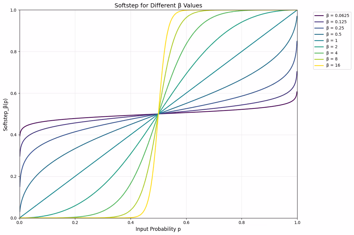
The “boundary” function $b(p)={\mathrm{𝟏}}_{p\ge \frac{1}{2}}$ can be smoothly approximated by a family of functions that sharpen/soften in logit-space and map back to probability space.

with $\beta \ge 0$ where $\beta$ represents the inverse-temperature parameter.

Notice the following:

By analogy with $F$ we can define

Notice,

What happens when we optimize $F_{\beta }$?

Let’s look at $ℒ=\frac{1}{2}(F_{\beta }-q{)}^2$:

Note that

Let $w_{t,\beta }={\mathrm{softstep}}_{\beta }^{\prime }(p_t)$.

And, assume there are $T$ positions in the sequence.

The only part here which depends on $p_t$ is $w_{t,\beta }$. To understand this non-uniform gradient pressure let’s graph ${\mathrm{softstep}}_{\beta }^{\prime }(p_t)$ for different inverse temperatures

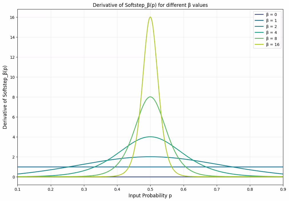
For moderate values we have a bump that’s centered around $\frac{1}{2}$. You can see as $\beta \to \infty$ it’s approaching a Dirac delta at $\frac{1}{2}$.

For $\beta =0$ we have a horizontal line at $0$: no gradients at all. For $\beta =1$ we have a horizontal line at $1$: no effective dependency on $p_t$. As $\beta \to \infty$ we approach the Dirac delta: only the exact value $\frac{1}{2}$ receives any gradient (measure zero), so effectively we get no gradient. As above, $F_{\infty }=F$ and we know $F$ isn’t differentiable, so this checks out.

For $\frac{\partial ℒ}{\partial p_t}$ with $\beta =1$, we push with the same magnitude on the $p$‘s until $F_1=G=q$.

For $\frac{\partial ℒ}{\partial p_t}$ with $\beta >1$, we push on $p$‘s until $F_{\beta }=q$, harder near the threshold. This causes a bit of polarization while getting $F_{\beta }$ on target.

In practice, moderate inverse temperature values like $\beta \in [2^1,2^4]$ seem to work fine.

Looking back at our gradient

Maybe we think the $w_{t,\beta }$ weight is nice and all, but in the end we want to get $F$ on target, not $F_{\beta }$. For moderate inverse temperatures these won’t be exactly the same.

So, what if we wanted a loss that both uses the $w_{t,\beta }$ but also keeps us on the hard target, i.e., such that

We can achieve this easily using the same trick as ${ℒ}_{\text{simple}}$:

Just as before, $F$ isn’t differentiable so its partial is irrelevant so only $\frac{\partial ℒ}{\partial F_{\beta }}$ matters, and we get what we need.

Notice that this is a generalization of ${ℒ}_{\text{simple}}$ (and therefore a generalization of Goomba’s original ratio loss) since $F_1=G$:

Values of $\beta$ just over $1$ allow us to nudge values away from $\frac{1}{2}$.

If, for whatever reason, we actually did want to constrain $G$ too we could do,

This also works fine and just shapes the distribution of $p$‘s a bit more. Benefits untested/unclear. But again, since $G$ can just be written in terms of $F_{\beta }$ it makes you wonder why we stop shaping the distribution here. Why not use multiple values of $\beta$? E.g., suppose our highest $\beta$ is $8$. Then we could do something overkill like

We’re doing the use-actual-hard-$F$-trick for the highest inverse temperature term and that last $F_1=G$.

There might be some benefit to adding the $G$ target term to ${ℒ}_{\beta }^{\text{new}}$, but I think the above is indeed overkill.

What’s the point of this generalization?

In a selfish mathematical sense it’s nice to realize $F$ and $G$ as one abstraction.

Practically, as mentioned, pushing harder on middling $p$‘s increases polarization. In my testing this manifests as moderately lower mean binary entropy and more stable ratio loss. I observe spikes in the original Goomba’s ratio loss (due to spikes in $F$). Fewer values straddling $\frac{1}{2}$ intuitively leads to more stable $F$.

Here is a tiny example training run comparison of two 2-stage models; blue is Goomba loss and red is ${ℒ}_4^{\text{new}}$. The top graph is comparing the $F$ values for stage 1 and the bottom graph is comparing the mean binary entropy for stage 1.

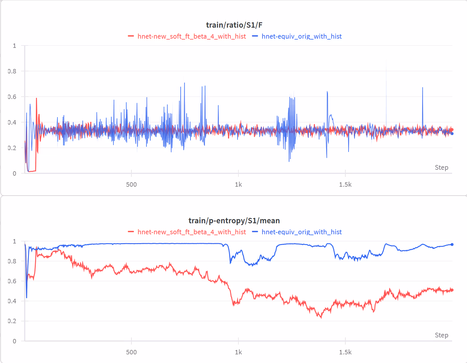
If binary entropy decreases naturally as a result of training then this stability shouldn’t be a problem later in training. Fine, in that case you can use a larger $\beta$ like $4$ or $8$ in the beginning of training and decay it smoothly to $1$ at which point it becomes identical in optimization behavior to the Goomba ratio loss. But, does entropy naturally fall during training?

The router’s binary entropy

The paper claims:

Mechanistically, although $F$ is not differentiable, the network can be trained toward targeted compression ratios through $G$, which provides continuous feedback.

When $F=G$, the loss attains a minimum of ${ℒ}_{\text{ratio}}=1$ when $F=G=\frac{1}{N}$. Interestingly, the loss can theoretically fall below 1 when $F\ne G$ (e.g., $F=\frac{1}{N}+\epsilon$ and $G=\frac{1}{N}-\epsilon$), which we indeed observe during training. Despite this theoretical possibility, the loss effectively guides the model toward the desired compression ratio in practice. In practice, as our architectural design encourages the routing module to make confident decisions (i.e., boundary probabilities approaching 0 or 1), $F$ naturally converges toward $G$, and the loss effectively guides the model toward the desired compression ratio.”

As mentioned, $F=G=q$ is not a minimum it’s a saddle point. And, as is clear from the form of their loss above, ${ℒ}_{\text{ratio}}=0$ when $F=q$ or when $G=q$. The gradient dies when $F$ attains its target; there is no gradient pressure from this ratio loss for $G$ to attain its target.

Let’s look at some actual stats for FineWeb-Edu on the checkpoints Goomba uploaded for hnet_1stage_L and hnet_2stage_L.

== H-Net batch setup (FineWeb-Edu) ==
batch_size: 256  max_len: 512  fineweb_name: sample-10BT

============ 2-stage ============
model_path:  ./hnet_2stage_L.pt
config_path: ./configs/hnet_2stage_L.json
n_compress:  1-3-9
CE_loss (nats/token): 0.573152
bpb (bits/byte):      0.826884
ratio_loss (sum):     2.044173
stage 1: F=0.350883  G=0.340252  ratio_loss=1.000546  H(p) mean=0.087364 bits  var=0.024160
stage 2: F=0.258758  G=0.203334  ratio_loss=1.043626  H(p) mean=0.218104 bits  var=0.120050
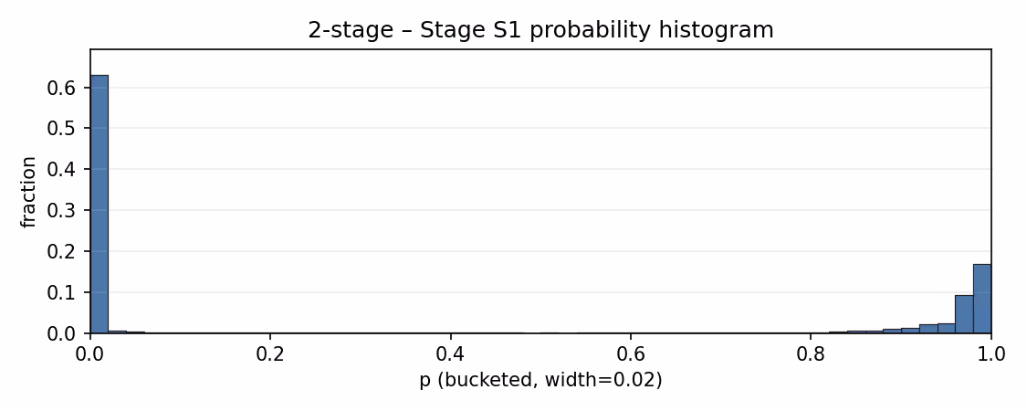
saved histogram: p_hist_2-stage_S1.png
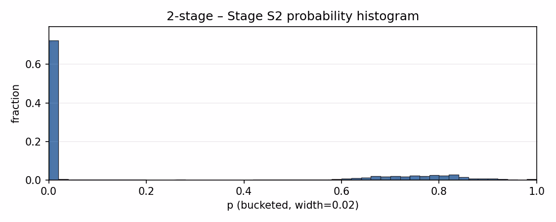
saved histogram: p_hist_2-stage_S2.png

============ 1-stage ============
model_path:  ./hnet_1stage_L.pt
config_path: ./configs/hnet_1stage_L.json
n_compress:  1-6
CE_loss (nats/token): 0.579933
bpb (bits/byte):      0.836667
ratio_loss (sum):     1.007449
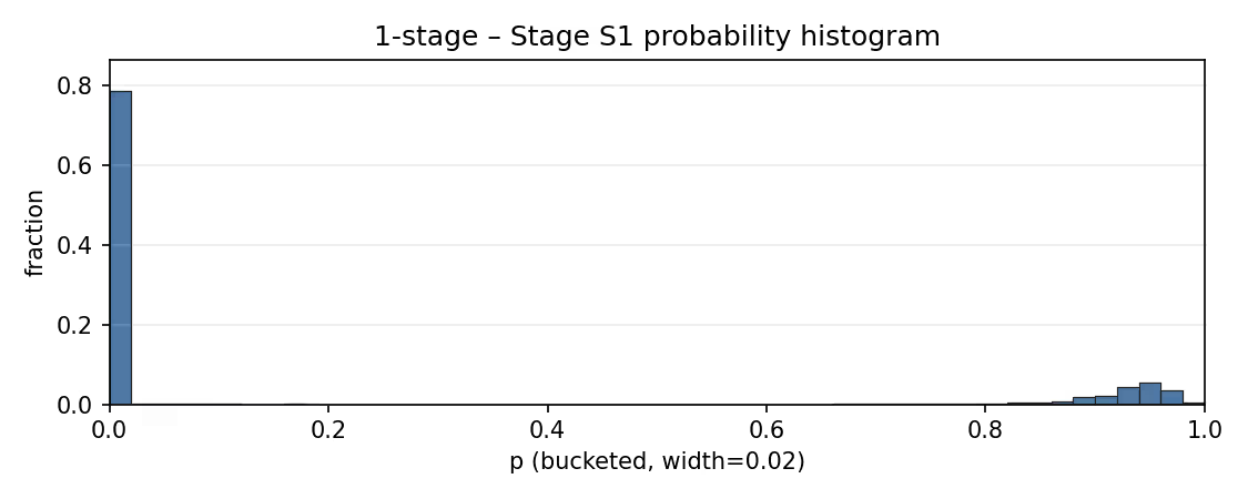
stage 1: F=0.207146  G=0.192224  ratio_loss=1.007449  H(p) mean=0.087115 bits  var=0.029150
saved histogram: p_hist_1-stage_S1.png

Do we see $F=G=q$ here? Eh, kinda.

The 2-stage model has a target of $q=\frac{1}{3}$ for both stages: the first stage of the 2-stage model looks closest; its second stage isn’t very close.

The 1-stage model has a target of $q=\frac{1}{6}$: it’s kinda close.

I included the mean and variance of the binary entropy of the $p$‘s. To understand what those “should” be let’s go over what happens when we optimize different quantities (not via SGD but just general optimization) subject to maximum mean binary entropy.

1. Optimize for $G=q$. We get the trivial solution that all $p$‘s are $q$, and therefore $F=0$. Training collapses. In particular if $q=\frac{1}{3}$ then the mean binary entropy $\overline{H(p)}\approx 0.918$ bits.

2. Optimize for $F=q$. We get $qT$ values which are $\frac{1}{2}+ϵ$ and $(1-q)T$ values which are $\frac{1}{2}-ϵ$. We get $G\approx \frac{1}{2}$ and the mean binary entropy $\overline{H(p)}$ approaches $1$ bit.

3. Optimize for both $G=q$ and $F=q$. The situation here is slightly more complex. The maximum entropy solution has $qT$ values at $\frac{1}{2}+ϵ$ and $(1-q)T$ values at $\frac{q}{2(1-q)}$. In particular substitute $T=300$ and $q=\frac{1}{3}$. We get $100$ values at $\frac{1}{2}+ϵ$ and $200$ values at $0.25$ for $F=\frac{1}{3}$, $G\approx \frac{1}{3}$ and $\overline{H(p)}\approx 0.8742$ bits. This entropy is only slightly less than option 1.

In practice with short training runs I find that Goomba’s H-Net setup resembles situation 2 early in training: the $p$‘s cluster around $\frac{1}{2}$ giving high mean entropy. It’s clear that their ratio loss has no mechanism for decreasing entropy. A decrease in entropy must come from the other gradient pressure on the $p$‘s: the EMA smoothing in the upsampler and the “confidence”-STE.

The 1-stage Goomba checkpoint has H(p) mean=0.087115 bits

And the 2-stage Goomba checkpoint has H(p) mean=0.087364 bits on the first and H(p) mean=0.218104 bits on the second stage.

These entropies are much lower than what I observe in short training runs. For longer training runs like Goomba’s I’d like to know: how do these binary entropies drop over time? Is it sudden or gradual?

Is it fair to call these “confident decisions (i.e., boundary probabilities approaching 0 or 1)”? eh. You can see that stage 2 of the 2-stage model has a fair mass in the $[0.6,0.8]$ region with a mean entropy of $\approx 0.22$ bits. Noticeably all these stages seem to be much more confident around $0$ than $1$, with significant mass in [$0.8,0.9]$.

The confidence score STE

Between the EMA smoothing in the upsampler and the “confidence scoring”, surely the latter is responsible for causing an entropy drop, right? I’m not so confident.

They define

I’ll make my own definition, which we can call the “distance to boundary function” or just “distance function”. For a given $p$ it just gives the distance to $0$ or $1$, whichever is less:

Then their confidence score can just be written as

The distance function has range $[0,\frac{1}{2}]$ and accordingly their confidence score has range $[\frac{1}{2},1]$. I find this definition simpler. More on this later.

In the upsampler, for each position $t$, they scale the most-recent EMA-smoothed $\hat{z}$ with $c(p_t)$. They use an STE such that $c$ appears to be $1$ in the forward pass. I.e.,

Let’s analyze the impact of this gradient on our $p$‘s. Let $y_t=\mathrm{Upsampler}(\tilde{z},c{)}_t$.

We have $\frac{\partial \mathrm{STE}(c_t)}{\partial c_t}=1$, so

Notice that the sign of $g_t$ can be positive or negative regardless of $b_t$. So all four cases are possible here. Polarization of $p$ doesn’t obviously pop out of this.

What if we wanted a stronger gradient closer to $\frac{1}{2}$ (and a weaker gradient closer to boundaries)? That might actually cause some polarization. I.e., what if we wanted

In that case we can just take

with range $[-\frac{1}{8},0]$. If we feel guilty about that range we can take

But, again, only the gradient actually matters. So let’s ignore the additive constants.

Now that we’re looking at it, why not tweak the coefficient on $c$ more thoroughly? This term doesn’t get used in the forward pass; the scaling on $c$ is analogous to a loss term coefficient. Goomba’s existing $c$ could just as well be written

for some positive coefficient $\gamma$. They used $\gamma =1$ but I doubt that’s optimal.

Let’s write our variant as

I haven’t tested this; I’m just demonstrating that their choice isn’t obviously better than nearby alternatives. This should be tested.

Interpreting the “confidence score”

Is it fair to call this a “confidence score”? To me it seems to be a stretch given that we’re only using the function for its derivative. We just want $\mathrm{sgn}(p_t-\frac{1}{2})$. That’s it.

If we interpret the gradients of the $p$‘s I think it’s possible to get an intuition for what its real effect is. To be fully explicit, let’s exhaust all cases. For simplicity ignore $g_t=0$ since it’s measure $0$ and assume we’re talking about a 1-stage H-Net.

1. $p_t\ge \frac{1}{2}$. This position is a boundary. The main network saw ${\hat{x}}_t$ when it produced ${\hat{z}}_t$. Scaling the smoothed version, ${\bar{z}}_t$ will either (locally) (net) decrease or increase the loss. Instead of scaling, we will interpret that as: decreases loss $\to$ increase $p_t$ so this boundary position is more likely, increases loss $\to$ decrease $p_t$ so this boundary position is less likely.

2. $p_t<\frac{1}{2}$. This position is not a boundary. The main network saw the most recent boundary as a proxy instead, i.e. ${\tilde{z}}_t$. Scaling the smoothed version, ${\bar{z}}_t$ will either (locally) (net) decrease or increase the loss. Instead of scaling, we will interpret that as: decreases loss $\to$ the proxy in this position is working out well (why ruin a good thing?) we should lower $p_t$ such that this position continues not being a boundary, increases loss $\to$ the proxy in this position isn’t working well, let’s maybe give this position a chance to be a boundary.

This confidence STE is just a heuristic. We don’t actually have the counterfactual world where the main network saw anything other than the boundary position ${\hat{x}}_t$‘s that it did.

Alternative “confidence score”-like heuristics

It’s easy to come up with other heuristics that sound just as plausible (if more complex to implement). Here are some ideas along those lines.

Notice that a position $t$ borrows from a previous boundary $r$ iff every position $i$ in $(r,t]$ has $p_i<\frac{1}{2}$.

You could replace the pointwise gate tweak with a structure‑aware credit assignment that follows the model’s realized routing. Two rough ideas

1. Pool feedback over each decision’s “region of responsibility” then nudge the entry decision up or down while counter‑nudging the interior positions based on whether that region helped or hurt

2. Trace feedback token‑by‑token along the actual route taken, weighting each position by how much the route depended on it

As with the alternative confidence score function above, I haven’t tested these ideas yet but it seems reasonable to me that they could improve over the confidence STE.

Directly penalizing high entropy

Recapping the above with regards to entropy,

• the Goomba ratio loss doesn’t decrease binary entropy

• Early training has high binary entropies; I observe $\approx 0.976\text{ bits}$ still after 3k steps.

• ${ℒ}_{\beta }^{\text{new}}$ will decrease entropy moderately early in training. For moderate $\beta$‘s I observe roughly $0.5$ to $0.75$ bits after a few thousand steps.

• By the end of Goomba training some emergent combination of EMA + confidence-scoring-STE has significantly decreased the entropies. They’re still not drastically low e.g. $<0.01$ bits.

An alternative we can try is to directly penalize high entropy. E.g., let

where $\mathrm{H}(p)$ is the binary entropy function.

Then we could introduce a new loss term

While this works mathematically, the gradients are largest near the boundaries (close to $0$ and $1$), which is counterproductive for our goal of polarization. We want exactly the opposite: strong gradients near $\frac{1}{2}$ and weak gradients near the boundaries. As an alternative we can use the square of the distance function from earlier.

Define:

This has zero gradients at the boundaries and maximal gradients near $\frac{1}{2}$ (the derivative is undefined exactly at $\frac{1}{2}$; not a problem in practice. ²)

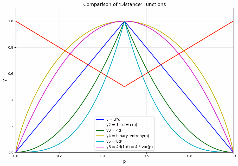
Here’s a visualization of (comparably-scaled versions of) various related functions so you can compare their shapes. I included the confidence function from earlier and the Bernoulli variance too, for comparison.

In my experiments this regularization term works, even with very low weights like ${\lambda }_{\text{ent}}=0.001$. Even if we only optimize $G$ e.g. with our ratio loss being $ℒ=(G-q{)}^2$ with no pressure on $F$ at all the inclusion of this regularization will rapidly (few hundred steps) decrease the entropy to something like $\approx 0.01$ to $0.02$ bits, and $F$ will be on target. Interestingly, I observed that the second stage entropy decreases much more gradually. While it will also go on target fine in a couple hundred steps, the drop in entropy is much more gradual after that (whereas stage 1 dips precipitously).

If we find this regularization too aggressive we can apply a margin loss where gradient pressure is only applied if the mean value exceeds some value corresponding to a binary entropy of, e.g. $0.1$ bits. This also works, but similar to the above, the second stage is much more stubborn about dropping below the margin. In my experiment the first stage entropy dropped well below the target but the second stage was slightly high.

Is forcing low entropy a good idea?

It seems plausible to me that artificially forcing low entropy in the router could harm learning. For example, artificially forcing low entropy could plausibly harm learning by causing the router to prematurely commit to a suboptimal routing strategy. It also seems plausible that it could help learning via the stability benefits. Needs more experiments at larger scales than I can manage. And in the tiny runs that I’ve done using just ${ℒ}_{\beta }^{\text{new}}$ I observe that the histogram of probabilities for the router is shifting around in shape drastically during training, despite the push towards moderate entropy. I predict that the moderate entropy drop early in training from using just ${ℒ}_{\beta }^{\text{new}}$ will be net neutral or mildly positive for final loss. I think the stability benefits are a win.

Cosine Q/K routing

I find it hard to believe that the Mamba2 layers in the encoder can’t easily find the inductive bias of the cosine Q/K routing in the paper. In the ablations in section 3.3 they mention using a head for routing (probably linear or MLP) but say the wild fluctuations in compression ratio harmed performance. The graphs in Figure 7 support that.

Seems plausible to me that some of the techniques in this post could be used to stabilize a linear or MLP router.

The Holy Grail: ‘natural’ gradients for the down/upsampling

The EMA smoothing seems fairly intuitive and motivated to me. I can also accept the ratio loss (at least my generalization of it): a target compression ratio is reasonable. But, the confidence-score-STE is clearly a hack. Unfortunately, as shown in the ablations, it clearly helps the final loss. It seems very plausible that there are alternative hacks which work even better.

But, is there an HNet-like architecture which has a better down/upsampling design with ‘natural’ gradients that fall out cleanly from the definition of the forward pass? (Which also outperforms H-Net). This is less clear to me. After all, MoE’s are basically a hack and afaik no one has an ‘elegant’ alternative.

I hope we find out!